Squishing a big bad bug
By Zhian N. Kamvar in R science
September 17, 2017
As I was preparing to push a new version of poppr to CRAN , this tweet (appropriately) came across my feed:
Mistakes happen in science. What matters is what you do next. Anyone want to share a story of a mistake & how they handled it?
— Adriana Porter Felt (@__apf__) September 10, 2017
The reason I was updating poppr was to fix a mistake I had made a few years ago. In the realm of scientific mistakes on a scale of hapliod to arsenic, I would say this probably falls somewhere on the lower end, but still significant enough that I felt I should blog about it ¯\_(ツ)_/¯.
My Mistake
Mistakes in scientific software happen all the time, which is why we have automated testing. Usually, these kind of bugs are things like simple logical errors that can easily be fixed by changing a single character. Unfortunately, the issue I was fixing was not so easily fixed. In short, in my assumptions about how to calculate Bruvo’s genetic distance for polyploid genotypes with multiple ambiguous alleles was incorrect (a detailed explanation of how Bruvo’s distance works can be found below for those interested). Without going into too much detail, at the heart of the error, I had fallen for a common statistical misconception of independent probabilities. Consider the following question:
If you have two fair coins and flip both of them, what is the most likely scenario?
- both are heads (🐦 , 🐦 )
- both are tails (🦅 , 🦅 )
- one heads and one tails (🐦 , 🦅 )
- all are equally likely (🐦 , 🐦 ) == (🐦 , 🦅 ) == (🦅 , 🦅 )
When I first saw this question, my immediate answer was d, but if I had paid attention in statistics class, or even remembered what the dots on my Settlers of Catan board meant, I would have answered c.
Embarassingly, I had assumed that the possible outcomes were unordered (the number of which is dictated by the multiset coefficient),
| outcome | probability |
|---|---|
| (🐦 , 🐦 ) | p |
| (🐦 , 🦅 ) | p |
| (🦅 , 🦅 ) | p |
as opposed to ordered (of which there is an exponential number of possible outcomes).
| outcome | probability |
|---|---|
| (🐦 , 🐦 ) | p |
| (🐦 , 🦅 ) | 2p |
| (🦅 , 🦅 ) | p |
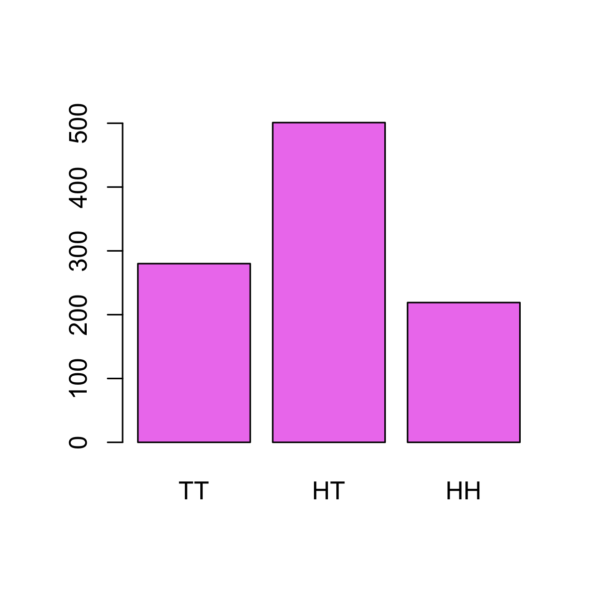
Of course, both (🐦 , 🦅 ) and (🦅 , 🐦 ) can occur with equal frequency. You can see this with a little simulation:
# Function to flip a coin N times
flip   <- function(n) sample(c(1, 0), n, replace = TRUE)
# Flipping two coins 1000 times each
n      <- 1000
set.seed(2017-09-23)
trials <- replicate(2, flip(n))
colnames(trials) <- c("coin 1", "coin 2")
rownames(trials) <- paste("trial", seq(n))
head(trials)
##         coin 1 coin 2
## trial 1      0      0
## trial 2      0      1
## trial 3      1      0
## trial 4      0      1
## trial 5      1      1
## trial 6      0      0
res        <- table(rowSums(trials))
names(res) <- c("TT", "HT", "HH")
barplot(res, col = "violet")
The Problem
The process to calculate Bruvo’s distance for polyploids with multiple ambiguous alleles involved taking the average value of the distance over all possible genotypes. The problem with my assumption of all possible unordered genotypes was that this fundamentally changed the structure of how I iterated through the possibilities, which meant that I would either have to completely re-write the machinery 😭 or find a clever way around it. 🤔
I chose the latter path 😤
The Solution
It turns out that you can calculate the number of possible combinations of a given set of items using the multinomial coefficient:
$$ \frac{n!}{k_1!k_2!…k_m!} $$
where n is the number of items in your set and each k represents the number of each unique item. Since Bruvo’s distance doesn’t take order into account when it calculates the distance, it was possible to multiply the distance at a particular allele combination with the multinomial coefficient and use the sum of the multinomial coefficients as the denominator to get the average distance1. In terms of the coin flips above, we can see how it would work:
| Replaced alleles | distance | coefficient |
|---|---|---|
| (🐦 , 🐦 ) | a | 1 |
| (🐦 , 🦅 ) | b | 2 |
| (🦅 , 🦅 ) | c | 1 |
The mean without the coefficient would be (a*b*c/3) whereas the mean with the coefficient would be (a*2b*c/4).
Implementation
Because I didn’t have to substantially change the architecture of the calculation, I was able to give poppr users the ability to compare their data by adding a switch in the internal functions that would turn the coefficient calculation off if desired.
This switch is controlled by the global option: options(old.bruvo.model = FALSE).
If it’s set to TRUE, calculation of Bruvo’s distance will revert to the old method of unordered alleles.
By doing this, I was able to avoid adding extra potentially confusing arguments to the functions that use Bruvo’s distance while still providing backwards compatibility. 👍
Conclusion
Mistakes in scientific software are commonplace. The very first bug discovered in poppr was discovered in 2014, there have been many more since, and there will be more as time goes on. When I find a mistake in poppr, I do what I would hope any other developer would do: I fix the mistake 🐛🔨, make a note that I fixed it 📝, and write a test to make sure the mistake never happens again 💻 ✅. If I make a mistake, I own it. There is no valor in covering it up, making excuses for it, or even fixing it and pretending it never happened.
Unfortunately, in this case, it took me several months from finding the bug to actually fixing it. This is due, in part, to the fact that I’m now only working on poppr in my spare time. It was also in part for the fact that it took me so long to even figure out the right terms to google for the multinomial coefficient. In terms of actual coding, I spent a weekend re-learning C and getting everything implemented.
At the end of the day, I figure that if I am open and transparent about how I fix bugs in poppr, then my users will hopefully have trust in me and also be comfortable in brining up any unexpected results they find.
Calculation of Bruvo’s distance
Bruvo’s distance is used for microsatellite markers assuming a stepwise mutation model. Between any two alleles the distance, \(d\), is
$$ d = 1 - 2^{-|x|} $$
where \(x\) is the number of repeat units between the alleles. For example, if you have two alleles, 420 and 428 with a repeat motif of ACAT, then they would represent (ACAT)$_{105}$ and (ACAT)$_{107}$, respectively, which would result in a distance of 0.75.
This gets more complicated when you increase the ploidy, because then you must find the minimum average distance among all the alleles. In practice, this involves creating a matrix of Bruvo’s distance for all alleles. So, for example, if you had the following alleles in two tetraploid samples:
| genotype 1: | 20 | 23 | 24 | 30 |
| genotype 2: | 20 | 24 | 26 | 43 |
The resulting genotype matrix would look like this:
| 20 | 23 | 24 | 30 | |
|---|---|---|---|---|
| 20 | 0.0000 | 0.875 | 0.9375 | 0.9990 |
| 24 | 0.9375 | 0.500 | 0.0000 | 0.9844 |
| 26 | 0.9844 | 0.875 | 0.7500 | 0.9375 |
| 43 | 1.0000 | 1.000 | 1.0000 | 0.9999 |
If you take the average of the diagonal, you end up with 0.5625. However, if we switch columns 2 and 3 in the above matrix, we find that the average is 0.4687. If we were to try all possible combinations of rearranging these columns and calculating the mean of the diagonal, we find that this is the minimum value. Because of this, order of alleles does not matter when calculating Bruvo’s distance. This fact becomes important in just a little bit.
Polyploid problem: partial heterozygotes
Of course, this is assuming that all alleles are known, but the problem with polyploids is that it is often difficult to accurately score genotypes that are only partially heterozygotic, so Bruvo came up with a solution where all possible combinations of the observed alleles are used to fill the missing genotypes as demonstrated in figure 1 of the publication:

This figure is a bit confusing to look at, but what it’s demonstrating is that if you weren’t able to score that “30” allele, you would be comparing three alleles against four. To compensate, you could do one of four things:
- Replace the allele with the three known alleles in that genotype (b)
- Replace the allele with the four known alleles of the other genotype (c)
- Replace the allele with infinity (d)
- Do 1 and 2 and average the results.
In calculating 1, 2, and 4, you must consider all possible combinations to
fill the missing allele. Luckily, when you only have one allele missing, all possible combinations amounts to the number of alleles observed. However, when you have more than one ambiguous allelic state, the question becomes, do you consider all possible ordered combinations of alleles, of which there are nk where n is the number of observed alleles and k, the number of ambiguous alleles or all possible unordered combinations, of which there are \({n+k-1}\choose{k}\) combinations.
For example, if you were comparing two genotypes:
| genotype 1: | 🤷 | 🤷 | 23 | 24 |
| genotype 2: | 20 | 24 | 26 | 43 |
you would need some way to replace the two ambiguous alleles (🤷) from genotype 1. If we assume that the extra alleles in genotype 2 are due to a recent genome expansion event (genome addition model), we would replace the ambiguous alleles with the observed alleles in genotype 1. Here are all the unordered combinations:
| genotype 1: | 23 | 23 | 23 | 24 |
| genotype 2: | 20 | 24 | 26 | 43 |
Table 1: Distance: 0.6875
| genotype 1: | 23 | 24 | 23 | 24 |
| genotype 2: | 20 | 24 | 26 | 43 |
Table 1: Distance: 0.6562
| genotype 1: | 24 | 24 | 23 | 24 |
| genotype 2: | 20 | 24 | 26 | 43 |
Table 1: Distance: 0.6562
If we take the average of the three, we get a Bruvo’s distance of 0.6667, but if we remember that there are two ordered combinations for the center genotype, we average over four distances to get 0.6641.
-
For those who like details, here’s the calculation of the multinomial coefficient and here’s how it was implemented in the genome addition model. ↩︎