Positive Contact

This version of poppr is a direct result of feedback that was prompted by my own feedback.

I’m always grateful for eagle-eyed users of poppr who report when things are going awry. Recently, I had noticed that poppr was cited in a recent review on the analysis of polyploid genetic data (Meirmans, Liu, and Tienderen 2018) that highlighted some limitations with established methods, including Bruvo’s distance (Bruvo et al. 2004).

I had noticed a pattern that I thought could have been caused by an old bug (that has since been fixed) and emailed Dr. Meirmans.

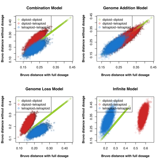
In the end, we figured that this pattern was genuine and not the result of a bug. However, my correspondence to Dr. Meirmans had prompted him to contact me about an upcoming paper he has on validating AMOVA for polyploids. He had noted that, while poppr worked well for calculating AMOVA, it failed to calculate the correct version of \(\rho\), which uses the AMOVA framework to assess differentiation in autopolyploids by calculating a distance matrix on individual-based allele frequencies ( Ronfort et al 1998). After a brief moment of embarassment, I got to work updating poppr and its documentation.

Changes in poppr version 2.7

Poppr version 2.7 introduces a change to how AMOVA is calculated and two new functions for data conversion:

• make_haplotypes() for splitting data into pseudo-haplotypes
• as.genambig() for converting genind/genclone objects to polysat’s genambig class.

The changes will be outlined here.

Note: Due to a documentation error, the correct version will be 2.7.1

AMOVA for polyploids

Meirmans and Liu (unpublished) present an analysis of the AMOVA framework for polyploids, showing that it is possible to calculate AMOVA for polyploiods if full dosage is known. Thus, poppr can now provide AMOVA calculations for polyploid data if the full dosage is known. If this is unknown (most cases), then the parameter \(\rho\) will be calculated ( Ronfort et al 1998).

Rho is a method of calculating population differentiation in the AMOVA framework without considering within-individual variance and is analogous to Fst for use with autotetraploid organisms ( Ronfort et al 1998; Miermans and Liu 2018). The process uses the Euclidean distance of allele frequencies and can be performed by setting within = FALSE.

library("poppr")
data("Pinf")
Pinf

## 
## This is a genclone object
## -------------------------
## Genotype information:
## 
##    72 multilocus genotypes 
##    86 tetraploid individuals
##    11 codominant loci
## 
## Population information:
## 
##     2 strata - Continent, Country
##     2 populations defined - South America, North America

# be sure to recode your polyploid data so that there are no zeroes for placeholders
(prc <- recode_polyploids(Pinf, newploidy = TRUE))

## 
## This is a genclone object
## -------------------------
## Genotype information:
## 
##    72 multilocus genotypes 
##    86 diploid (55) and triploid (31) individuals
##    11 codominant loci
## 
## Population information:
## 
##     2 strata - Continent, Country
##     2 populations defined - South America, North America

# calculate rho
rho  <- poppr.amova(prc, ~Continent/Country, within = FALSE, cutoff = .1, quiet = TRUE)
rho$statphi

##                              Phi
## Phi-samples-total     0.12713922
## Phi-samples-Continent 0.05269217
## Phi-Continent-total   0.07858802

Here, the value of \(\rho\) is 0.1271392.

Changes in AMOVA for poppr 2.7 can affect your results

The process of calculating AMOVA in poppr involved four steps:

1. If the data were diploid, genotypes were split into pseudo-haplotypes
2. A distance matrix was calculated using diss.dist() and the square root was taken
3. The matrix and hierarchy were prepared for either ade4 or pegas
4. AMOVA was calculated using either ade4 or pegas

In this new version of poppr, you now have access to the function that splits haplotypes called make_haplotypes().

The major change in poppr 2.7 is that the dist() has replaced diss.dist()

Changing diss.dist() to dist()

The default distance calculation for all AMOVA was diss.dist(), which is a dissimilarity distance. For haploid or pseudo-haploid data, this is equivalent to a squared Euclidean distance, and was appropriate for calculating the distance for use when the within = TRUE option was set (which was default). This method, however, was not appropriate when not considering within-individual variation.

For example, this is how the previous versions of poppr would have calculated \(\rho\):

dissim <- diss.dist(prc)
old  <- poppr.amova(prc, ~Continent/Country, within = FALSE, cutoff = .1, quiet = TRUE, 
                    dist = dissim, squared = TRUE)

## Distance matrix is non-euclidean.

## Using quasieuclid correction method. See ?quasieuclid for details.

old$statphi

##                              Phi
## Phi-samples-total     0.15032208
## Phi-samples-Continent 0.12439575
## Phi-Continent-total   0.02960965

If we compare this result to the one above, we can see that there is a distinct difference in the values of \(\rho\).

AMOVA with missing data

The dist() function handles missing data differently than diss.dist(), so you may see small differences in your results (for details, see this StackOverflow answer: https://stackoverflow.com/a/18117751/2752888).

For example, the nancycats data set has an average of 2.3% missing data. This results in a small shift in the \(\Phi\) statistics. Here are the results with version 2.7:

data(nancycats)
strata(nancycats) <- data.frame(colony = pop(nancycats))
new <- poppr.amova(nancycats, ~colony, cutoff = .1, quiet = TRUE)

## Distance matrix is non-euclidean.

## Using quasieuclid correction method. See ?quasieuclid for details.

new$statphi

##                          Phi
## Phi-samples-total  0.1971382
## Phi-samples-colony 0.1235778
## Phi-colony-total   0.0839327

To show the results from previous versions, we need to use the new make_haplotypes() function to create pseudo-haplotypes:

nanhaps <- make_haplotypes(nancycats)

# confirm that the number of individuals is double that of the original data
nInd(nanhaps)

## [1] 474

2 * nInd(nancycats)

## [1] 474

# calculate squared Euclidean distance
d2n <- diss.dist(nanhaps)

# calculate AMOVA
old <- poppr.amova(nanhaps, ~colony/Individual, cutoff = .1, quiet = TRUE, 
                   dist = d2n, squared = TRUE)

## Distance matrix is non-euclidean.

## Using quasieuclid correction method. See ?quasieuclid for details.

old$statphi

##                           Phi
## Phi-samples-total  0.19292024
## Phi-samples-colony 0.12109840
## Phi-colony-total   0.08171772

The different treatment of the missing data has created a difference of 0.004218 in \(\Phi_{ST}\).

Converting genind/genclone to polysat

Polysat is a package that works with polyploid microsatellite data. You can install it from CRAN with install.packages("polysat"). The poppr function as.genambig() will convert from genind to genambig:

library("polysat") # load polysat
Pinf

## 
## This is a genclone object
## -------------------------
## Genotype information:
## 
##    72 multilocus genotypes 
##    86 tetraploid individuals
##    11 codominant loci
## 
## Population information:
## 
##     2 strata - Continent, Country
##     2 populations defined - South America, North America

Pinf.ga <- as.genambig(Pinf) # Convert to genambig
summary(Pinf.ga)             # Show the summary of the contents

## Dataset with allele copy number ambiguity.
## Insert dataset description here.
## Number of missing genotypes: 10
## 86 samples, 11 loci.
## 2 populations.
## Ploidies: 2 3 NA
## Length(s) of microsatellite repeats: NA

Once you have your genambig object, you can use all the functions polysat has available.

References

Patrick G Meirmans, Shenglin Liu, Peter H van Tienderen; The Analysis of Polyploid Genetic Data, Journal of Heredity, Volume 109, Issue 3, 16 March 2018, Pages 283–296, https://doi.org/10.1093/jhered/esy006

BRUVO, R., MICHIELS, N. K., D’SOUZA, T. G. and SCHULENBURG, H. (2004), A simple method for the calculation of microsatellite genotype distances irrespective of ploidy level. Molecular Ecology, 13: 2101–2106. https://doi.org/10.1111/j.1365-294X.2004.02209.x

Ronfort, Joëlle, Eric Jenczewski, Thomas Bataillon, and François Rousset. “Analysis of population structure in autotetraploid species.” Genetics 150, no. 2 (1998): 921-930. http://www.genetics.org/content/150/2/921.short